Individual Assignment 2: Traffic Assignment

Due Nov. 27 - Submit on Canvas

Points are assigned both on the correctness of the answer and the completeness of the solution – state all assumptions. Show all calculations and equations. Do not use Excel or other software packages.

Problem 1. Consider the simple network in the below figure where there are 100 vehicles per hour travelling from A to X and 500 from B to X. The travel time versus flow relationships (volume-delay functions) are depicted in the figure in minutes and the flow v in vehicles per hour.

a. Express the objective function of the mathematical program corresponding to Wardrop’s user equilibrium in terms of the flows and travel time-flow relationships in the figure. Hint: refer to the Traffic Assignment lecture slides.

b. Calculate the equilibrium flows on each link and the travel time for each group of travelers. Calculate the value of the objective function above under equilibrium conditions – i.e., the total expenditure in travel time on the network in veh-hr. You should start with an incremental assignment. You can assume the following loading: 50% A->X, 50% B->X, 50% B->X, 50% A->X. You should then use an all-or-nothing assignment as your second volume in the Frank-Wolfe (FW) algorithm. Perform only one FW iteration. You can use the same FW approximation as in the class example – i.e., evaluate \(\lambda\) = 0, 1/3, 2/3, and 1.

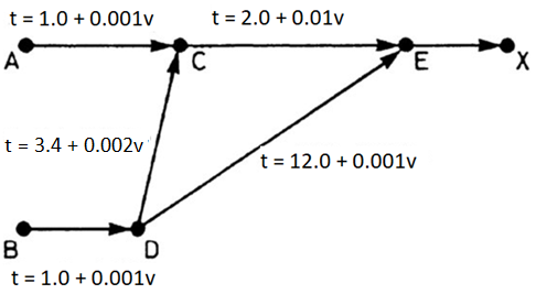
c. Local traffic engineers have decided to install speed restrictions on link C->D so that the new travel time versus flow function is: t=5.2+0.002v

The total expenditure in travel time (veh-hr) in the system is less than in (b) under these conditions. Why would this be the case? The following two tables show the final Frank-Wolfe flow results for the relationships in part (b) and (c), respectively. Please use these tables in your response.

Index	Arc	Fixed Cost	Variable Cost	Flow
0	A	C	1	0.001	100
1	B	D	1	0.001	500
2	C	E	2	0.01	569.23
3	D	C	3.4	0.002	469.23
4	D	E	12	0.001	30.77
5	E	X	0	0	600

Index	Arc	Fixed Cost	Variable Cost	Flow
0	A	C	1	0.001	100
1	B	D	1	0.001	500
2	C	E	2	0.01	430.77
3	D	C	5.2	0.002	330.77
4	D	E	12	0.001	169.23
5	E	X	0	0	600

Problem 2. Problem 1 assumes that traffic assignment is deterministic. In reality, traffic assignment (route choice) varies across decision-making motorists on the road.

a. Comment on possible reasons for stochasticity in route choice.

b. One way to handle stochastic traffic assignment is via discrete choice models. How might this face a computational challenge? You should support your response with a diagram. Examples and scenarios are also welcome additions.